About two weeks ago, a fire at a Tyson meat packing plant destroyed about 5 to 6% of the nation’s beef processing capacity. The fire caused a significant drop in the price of cattle and a significant rise in the price of wholesale beef, increasing the packing margin (the difference between cattle prices and beef prices). This has caused a lot of consternation. Here’s an excerpt from a recent article in the LA Times:
“Beef-packer margins rose to $378.25 per animal on Monday, an all-time high in HedgersEdge data. That’s more than double the levels reported just a week ago. Wholesale prices surged to $2.3869 a pound Friday, the highest in two years. Meanwhile, cattle prices on cash markets crashed to $1.0865 a pound on Friday, the lowest for this time of year in nearly a decade.
“These guys are making more money than they ever have,” Gary Morrison, vice president at commodity researcher Urner Barry, said of meatpackers.”
The packers may well be making more money, but these economic effects are exactly what one would expect even in a perfectly competitive market. It’s the first week of school here at Purdue, so I thought I’d get a little wonky and walk through some basic supply-demand graphs related to the so-called marketing margin.
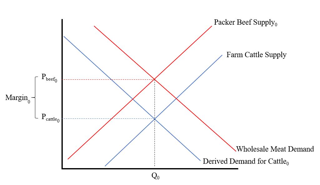
First, consider the situation before the fire, as shown in the figure below. Restaurants and grocery stores want beef to feed their customers, and this results in a demand for wholesale beef (this is given by the red downward sloping line labeled “Wholesale Meat Demand”). Packer’s acquire cattle, process them, and supply beef to the wholesale market, and this relationship is given by the red upward sloped line labeled “Packer Beef Supply0”. The intersection of these two lines determines the wholesale price of beef, Pbeef0.
Because packers need cattle to supply beef to the retail market, they have a “derived demand” for cattle given by the downward sloping blue line labeled “Derived Demand for Cattle0.” Cattle producers supply cattle to the market (as described the upward sloping blue line marked “Farm Cattle Supply”). The intersection of these last two lines determines the price of cattle, Pcattle0.
The difference in the wholesale price of beef, Pbeef0, and the price of cattle Pcattle0, is the marketing margin, Margin0. The way I’ve drawn the graph, there is 1 lb of wholesale beef for every 1 lb of cattle (something economist call “fixed proportions”), and this quantity is Q0.
Ok., now the fire happens and reduces the ability of packers to supply beef. This shifts the packer supply curve upward and to the left. As we can see in the figure below, the result is that wholesale beef prices will rise from Pbeef0 to Pbeef1.

But, that’s only part of the story. In addition to packer’s supply curve shifting, they also don’t need as many cattle (because they no longer have the capacity to process them). As a result, the derived demand for cattle by the packers also falls as shown in the following figure.
The result is that cattle prices fall from Pcattle0 to Pcattle1. As a result, the quantity of cattle/beef sold falls from Q0 to Q1, and the marketing margin increases from Margin0 to Margin1.

In short, the effects we’re seeing right now in the beef and cattle markets are exactly what we’d expect from a textbook treatment of a reduction in wholesale supply in a vertically linked market.
By the way, I’ll note that it is also possible to use this unexpected reduction in packer supply to estimate the elasticity of wholesale demand for meat. Why? The demand for wholesale meat hasn’t shifted, and so any price changes must be occurring because of movements along this curve, which gives us an estimate of the slope of the curve.
The formula for the elasticity of demand is (% change in quantity)/(%change in price). Assuming the supply curve is perfectly inelastic in the short run (unlike what I’ve draw above), the (% change in quantity) = -6% according to most news accounts. The current boxed beef price is about $2.42/lb for choice beef, up about 13% from $2.14/lb before the fire. Putting it together, the elasticity of wholesale demand for beef is = (% change in quantity)/(%change in price) = -6%/13% = -0.46, which seems imminently reasonable.
Addendum. After posting the above information yesterday, I’ve had a number of emails and comments. Some have pointed out that cattle slaughter numbers are actually up a bit since the fire. Doesn’t that contradict the above model? Here are a few thoughts.
There may have been some underutilized capacity in other plants that ramped up given the change in economic incentives. If so, this will ultimately push prices back closer to pre-fire levels when the dust settles. Still, we wouldn’t expect a complete reversion to “normal” (whatever that is) because this extra slaughter is now occurring in areas that presumably weren’t as efficient as was the case pre-fire.
It’s hard to know the counter-factual. Maybe there were already seasonal or economic issues that would have led to the an increase commercial slaughter during this time period anyway. So, yes slaughter numbers may have increased in the days following the fire, but the numbers may be still less than what was expected given current inventory and other factors.
There may be regional shifts and effects going on. Even if total industry capacity wasn’t affected, all those cattle that were geared up to go to the plant in Garden City need to be shipped elsewhere (presumably at higher transportation costs, which reduces their value).
No doubt, there are other factors too. The above model is a very simplified depiction of reality. There may be market power issues (but as the model above shows, the prices changes observed don’t require this explanation but they don’t rule it out either) or other dynamics occurring on top of these underlying forces. For example, a lot of cattle are sold based on some formula or contract price, which is likely to create frictions in price discovery that aren’t reflected in the above graph.