Senate Hearing on Livestock and Poultry Issues

Yesterday I had the opportunity to testify before the U.S. Senate Committee on Agriculture, Nutrition, and Forestry in a hearing about livestock and poultry. A video of the entire hearing is here. My written testimony is also at the link. For convenience, I’ve also reproduced it below.

Chairman Roberts, Ranking Member Stabenow, and Members of the Committee, thank you for inviting me here today.  I serve as Distinguished Professor and Head of the Agricultural Economics Department at Purdue University, and I will focus my remarks on six economic issues currently facing livestock and poultry industries: global protein demand and trade, mandatory price reporting, competition, labor, animal disease, and the need for innovation.

 Population and income are two key drivers affecting demand for meat and poultry. Slow population growth and concerns about an economic slowdown indicate the potential for depressed meat demand in this country.  Health, environment, and animal welfare criticisms, coupled with emerging plant- and lab-based competitive alternatives, are also significant headwinds. 

 These factors suggest that meat demand growth is largely expected to occur outside the United States.  Having access to consumers in other countries has become increasingly important to the livelihood of U.S. livestock and poultry producers. The U.S. exported about 12% of beef, 22% of pork, and 16% of poultry production last year.  It is in this context that trade agreements are important to help open markets for US producers to allow products to flow to consumers who value them most.

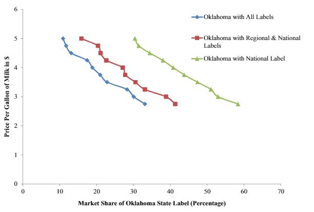
 Some U.S. producers have expressed concerns about the competition from imports, but the U.S. is a net exporter of meat and poultry products, and the types and qualities of meat we import tend to differ from what we export. There have been some calls to renew Mandatory Country of Origin Labeling (MCOOL).  Congress repealed MCOOL for beef and pork in 2015 to avoid more than $1 billion in retaliatory tariffs after a protracted legal battle with other countries before the World Trade Organization.  Our survey and experimental research suggests many consumers indicate they are willing to pay premiums for U.S. meat products; however, research also shows few consumers were aware of actual origin labels when grocery shopping, and analysis of grocery store scanner data did not reveal any significant changes in consumer demand for beef or pork after the implementation of MCOOL.  Meat demand indices indicate, if anything, beef and pork demand has increased after the repeal of MCOOL.  Cattle prices fell shortly after the repeal of MCOOL, but this is largely explained by an increase in cattle inventory that happened to coincide with the labeling policy change.  To the extent consumers are truly willing to pay a premium for U.S. labeled meat that exceeds the costs of tracing and labeling, there remain opportunities for private entities to take advantage of this market opportunity.

 The current authority for Livestock Mandatory Reporting (LMR) is set to expire in 2020.  LMR was designed to improve transparency, facilitate market convergence, and reduce information asymmetries.  Despite these laudable goals, academic research on impacts of LMR is mixed.  Shortly after its initial passage in 1999, surveys of cattle producers suggest expectations about the impacts of LMR may have been overly optimistic.  Some concerns have been expressed that LMR might facilitate rather than curtail anticompetitive behavior among packers.  However, evidence indicates LMR helped facilitate integration of regional markets.  It is important for LMR to continue to modernize and be agile in response to the pace of change in the industry.  One challenge is the dwindling share of cattle and hogs sold in negotiated or cash markets, which typically serve as the base price in formula contracts.  There are significant benefits to formula contracts and more producers are voluntarily choosing this method of marketing over the cash market, but questions remain about the volume of transactions needed in the cash market to facilitate price discovery.  A benefit of LMR is the massive amounts of data provided to economists and industry analysts to help understand these and other market dynamics.   

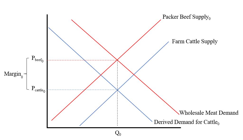
 Last month, price dynamics following a fire at a packing plant in Western Kansas renewed discussion about packer concentration and potential anti-competitive behavior. Concerns about anti-competitive behavior in general must be evaluated on a case-by-case basis, and details about this particular case are still emerging in light of simultaneous market dynamics that were also at play.  Available evidence to date suggests the observed reduction in cattle prices and the increase in wholesale beef prices following the fire are not inconsistent with a model of competitive outcomes. An unexpected reduction in processing capacity reduces demand for cattle, thereby depressing cattle prices. The need to bring in additional labor to increase Saturday processing and temporarily re-purposing cow plants for steers and heifers involves additional costs that pushed up the price of wholesale beef.  These price dynamics are not surprising and are generally what would be expected from the fundamental workings of supply and demand. 

 In general, a lack of availability of labor at processing facilities and in transportation have proved significant hurdles for the sector.  When processors are unable to secure sufficient workforce to operate facilities at capacity, there is the potential to reduce demand for livestock and poultry, which has much the same price effects witnessed after the Kansas fire.  

 I also urge the committee to pay close attention to emerging animal disease issues. African Swine Fever (ASF) in China has had a decimating impact on their hog herd and has increased their pork prices by almost 50%. The significant disruption to the Chinese hog supply has reverberated through global agricultural markets, reducing demand for U.S. soybeans and inducing substitution toward alternative proteins such as beef and poultry. While U.S. hog producers have been able to increase exports to China as a result of ASF, exports are not what they could have been had China not raised tariffs on pork.  It appears that ASF is spreading beyond China.  My calculations suggest that if an outbreak of ASF similar in relative magnitude to the one in China were to occur here, U.S. pork producers could lose about $7 billion/year and U.S. consumer harm would be at least $2.5 billion/year.  ASF is not the only animal disease concern, and an outbreak of foot mouth disease, discovery of bovine spongiform encephalopathy (BSE), or a return of avian influenza or Newcastle disease could have similar devastating impacts.  Thus, there is a need for additional funding for research to combat foreign animal disease. 

 There is also a need for funding to improve the productivity of the livestock and poultry sectors. Productivity growth is the cornerstone of sustainability.  For example, had we not innovated since 1970, about 11 million more feedlot cattle, 30 million more market hogs, and 7 billion more broilers would have been needed to produce the amount of beef, pork, and chicken U.S. consumers actually enjoyed in 2018.  Innovation and technology saved the extra land, water, and feed that these livestock and poultry would have required, as well as the waste and greenhouse gases that they would have emitted.  Investments in research to improve the productivity of livestock and poultry can improve producer profitability, consumer affordability, and the sustainability for food supply chain. 

What Food Policies do Consumers Like and Dislike?

I have a new working paper with Vincenzina Caputo in which we elicit consumers’ preferences for 13 different food policies. Here’s our main motivation (references removed for readability).

“A variety of food policies have been proposed, and in some cases enacted, in an effort to improve public health, environmental outcomes, or food security. Proposed actions include a spectrum of policies ranging from fiscal incentives/disincentives, bans, labelling programs, and passive policies such as subsides and investments in education. What food policy proposals do consumers prefer? While there have been numerous studies aimed at calculating the welfare effects of individual food policies it is difficult to easily ascertain the relative preferability of numerous policy options, even those that have the same objective (e.g., “fat taxes” and nutritional education both aim to improve public health). ”

We conducted a nationwide survey of 1,056 U.S. consumers who were asked to indicate the relative desirability of the following food policies.

Rather than use a traditional approach, where respondents are not required to make trade-offs between policies (e.g., people can approve of all policies or rank all policies as “very important”), we used the “best worst scaling” approach that requires respondents to make trade-offs. The approach requires respondents to answer a series of questions like the one below, where for each question, they have to indicate their most and least preferred policies.

The results are analyzed using a choice model that allows for preference heterogeneity. The main outcomes are below, reported as “preference shares” - i.e., the percent of people predicted to choose each policy as most preferable. Results indicate the highest levels of support for investments in agricultural research and requirements of food and agricultural literacy standards in public education. Fat, calorie, and soda taxes are the least popular. These preference shares provide a measure of intensity of preference in a population. Funding for agricultural research is 14%/8% = 1.75 times more preferable than symbolic nutritional labeling.

While the above results are useful in providing intensity of relative preferences, they do not indicate whether people would actually vote in favor of a policy. The table below shows the results of that question; the results largely align with the best-worse scaling approach. Fewer than one-third of respondents are in favor of these three tax policies.

There are a number of significant demographic correlates with policy preferences. Some are not surprising. For example, Nutrition Assistance (or SNAP) is more desirable to lower income vs. higher income households and Democrats vs. Republicans. As another example, soda taxes are less desirable among lower income households.

Funding for agricultural research was generally supported across all demographic categories except for age: older individuals were more supportive of funding for agricultural research than younger individuals.

The Cost of Slow Growth Chickens

I’ve had a couple previous posts on both the supply of and demand for slower growing chickens. There have been increasing calls for retailers to switch to slower growing breeds (often, older “heritage” breeds), with the presumptive aim to increase animal welfare and taste. The downside is that it is more expensive to produce chicken with these older breeds. The Journal of Agricultural and Resource Economics has now published a paper I co-authored with Nathan Thompson at Purdue University and Shawna Weimer, an assistant professor of poultry science at the University of Maryland on the costs for individual producers switching to slower growing breeds and the market impacts we project would occur if the entire industry did the same. This is an updated and peer-reviewed version of the paper I previously blogged about.

Here is the abstract:

“There has been substantial productivity growth in the broiler industry; however, high growth rates might adversely affect animal welfare, resulting in calls for slow-growth breeds. This research shows production costs are 11%–25% per pound higher for slower-growing breeds than for modern breeds, depending on the target endpoint. Breakeven wholesale price premiums needed equate net returns of slow- to fast-growth broilers range from $0.10/lb to $0.36/lb. Annual costs of an industry-wide conversion to slow growth are $450 million for consumers and $3.1 billion for producers. Consumer willingness-to-pay would need to increase 10.8% to offset the producer losses.”

Don’t like some of our assumptions? We’ve also created an excel-based tool that allows the user to change assumptions about input and output prices, as well as other model parameters, and see how costs and optimal days of feed change for faster and slower growing breeds. The tool dynamically updates figures like the one below. Try it for yourself!

My State is Better than Yours: Competition between State Food Branding Programs

The journal Agribusiness just released a new paper I co-authored with Clint Neill and Rodney Holcomb. The work was motivated by the observation that every state in the U.S. has an agricultural marketing program aimed at promoting foods from their state. Examples include the “Taste NY” and “Pride of New York” programs as well as “Go Texan” and “California Grown.”

Our questions were two fold: 1) How much do consumers value products labeled with their state’s logo relative to other states’ products, and 2) what are the implications for state marketing programs?

We surveyed 6,900 consumers in an eight‐state contiguous region. For our application, we chose milk, and asked people which of several milk products with different state logos (and a regional or national brand) they preferred at different prices.

Not surprisingly, we find that consumers prefer products with their own state’s logo. For example, Texans’ average willingness-to-pay (WTP) for Texas milk is $4.14/gallon, but Texans’ value for milk from bordering states, New Mexico, Oklahoma, and Arkansas only averaged $1.82, $2.65, and $2.72/gallon, respectively. There are a number of interesting patterns. Here’s an excerpt from the text:

“While each state’s consumers tend to prefer their own label and have a distinct order of preference for other states, the asymmetry between states is less clear. For example, Oklahoma consumers are willing to pay $2.84 for the Texas label but Texas consumers are only willing to pay $2.65 for the Oklahoma label, so there is an asymmetry of $2.84−$2.65 = $0.19. Thus, Oklahomans value the Texas label $0.19 more than Texans value the Oklahoma label.

Table 5 shows this type of asymmetry for all combinations. Interestingly, every other state’s consumers value the Colorado label more than Colorado consumers value other states’ labels. Alternatively, New Mexico consumers value all other state brands more than the other states’ consumers value the New Mexico label.”

While it is perhaps obvious that people in a state will tend to prefer their own products, it is also important to note that people have some value from agricultural products from other states (and, in fact, some small share of people prefer products from another state). The result is that state branding programs “steal” consumers from other states (the effect is a bit like the prisoner’s dilemma problem). The state branding program looks great if your the only state that has the program, but if all states have their own programs, the effects partially serve to cancel each other out. Here’s what we write about this so-called “beggar thy neighbor” effects:

“In the case of market shares, we were able to illustrate the large decreases as a group of producers from one state starts with having no state branded competitors to competing against several other brands within a region. Producers, ideally, would have a higher return if they were the only ones with a state label, but the optimal strategy for all agents in the region is to utilize a state label. Thus, the potential beggar‐thy‐neighbor scenario is possibly a Nash equilibrium. Furthermore, states who market their brand outside their borders are shown to have increased total market share”

For example, below is a graph showing what happens to demand for milk with a “Made in Oklahoma” label when no other states label their product (the green line with triangle markers) relative to what happens to demand for “Make in Oklahoma” milk when other states introduce their own labels (the red and blue lines). As the figure below shows, the market share more than halves when one state’s label has to compete with all the others in a region.

One potential solution (at least from the producer’s perspective) we discuss is for groups of states to band together and use a regional label.

The Economic of Packing Plant Fires and Cattle Prices

About two weeks ago, a fire at a Tyson meat packing plant destroyed about 5 to 6% of the nation’s beef processing capacity. The fire caused a significant drop in the price of cattle and a significant rise in the price of wholesale beef, increasing the packing margin (the difference between cattle prices and beef prices). This has caused a lot of consternation. Here’s an excerpt from a recent article in the LA Times:

“Beef-packer margins rose to $378.25 per animal on Monday, an all-time high in HedgersEdge data. That’s more than double the levels reported just a week ago. Wholesale prices surged to $2.3869 a pound Friday, the highest in two years. Meanwhile, cattle prices on cash markets crashed to $1.0865 a pound on Friday, the lowest for this time of year in nearly a decade.

“These guys are making more money than they ever have,” Gary Morrison, vice president at commodity researcher Urner Barry, said of meatpackers.”

The packers may well be making more money, but these economic effects are exactly what one would expect even in a perfectly competitive market. It’s the first week of school here at Purdue, so I thought I’d get a little wonky and walk through some basic supply-demand graphs related to the so-called marketing margin.

First, consider the situation before the fire, as shown in the figure below. Restaurants and grocery stores want beef to feed their customers, and this results in a demand for wholesale beef (this is given by the red downward sloping line labeled “Wholesale Meat Demand”). Packer’s acquire cattle, process them, and supply beef to the wholesale market, and this relationship is given by the red upward sloped line labeled “Packer Beef Supply0”. The intersection of these two lines determines the wholesale price of beef, Pbeef0.

Because packers need cattle to supply beef to the retail market, they have a “derived demand” for cattle given by the downward sloping blue line labeled “Derived Demand for Cattle0.” Cattle producers supply cattle to the market (as described the upward sloping blue line marked “Farm Cattle Supply”). The intersection of these last two lines determines the price of cattle, Pcattle0.

The difference in the wholesale price of beef, Pbeef0, and the price of cattle Pcattle0, is the marketing margin, Margin0. The way I’ve drawn the graph, there is 1 lb of wholesale beef for every 1 lb of cattle (something economist call “fixed proportions”), and this quantity is Q0.

Ok., now the fire happens and reduces the ability of packers to supply beef. This shifts the packer supply curve upward and to the left. As we can see in the figure below, the result is that wholesale beef prices will rise from Pbeef0 to Pbeef1.

But, that’s only part of the story. In addition to packer’s supply curve shifting, they also don’t need as many cattle (because they no longer have the capacity to process them). As a result, the derived demand for cattle by the packers also falls as shown in the following figure.

The result is that cattle prices fall from Pcattle0 to Pcattle1. As a result, the quantity of cattle/beef sold falls from Q0 to Q1, and the marketing margin increases from Margin0 to Margin1.

In short, the effects we’re seeing right now in the beef and cattle markets are exactly what we’d expect from a textbook treatment of a reduction in wholesale supply in a vertically linked market.

By the way, I’ll note that it is also possible to use this unexpected reduction in packer supply to estimate the elasticity of wholesale demand for meat. Why? The demand for wholesale meat hasn’t shifted, and so any price changes must be occurring because of movements along this curve, which gives us an estimate of the slope of the curve.

The formula for the elasticity of demand is (% change in quantity)/(%change in price). Assuming the supply curve is perfectly inelastic in the short run (unlike what I’ve draw above), the (% change in quantity) = -6% according to most news accounts. The current boxed beef price is about $2.42/lb for choice beef, up about 13% from $2.14/lb before the fire. Putting it together, the elasticity of wholesale demand for beef is = (% change in quantity)/(%change in price) = -6%/13% = -0.46, which seems imminently reasonable.

Addendum. After posting the above information yesterday, I’ve had a number of emails and comments. Some have pointed out that cattle slaughter numbers are actually up a bit since the fire. Doesn’t that contradict the above model? Here are a few thoughts.

1. There may have been some underutilized capacity in other plants that ramped up given the change in economic incentives. If so, this will ultimately push prices back closer to pre-fire levels when the dust settles. Still, we wouldn’t expect a complete reversion to “normal” (whatever that is) because this extra slaughter is now occurring in areas that presumably weren’t as efficient as was the case pre-fire.

2. It’s hard to know the counter-factual. Maybe there were already seasonal or economic issues that would have led to the an increase commercial slaughter during this time period anyway. So, yes slaughter numbers may have increased in the days following the fire, but the numbers may be still less than what was expected given current inventory and other factors.

3. There may be regional shifts and effects going on. Even if total industry capacity wasn’t affected, all those cattle that were geared up to go to the plant in Garden City need to be shipped elsewhere (presumably at higher transportation costs, which reduces their value).

No doubt, there are other factors too. The above model is a very simplified depiction of reality. There may be market power issues (but as the model above shows, the prices changes observed don’t require this explanation but they don’t rule it out either) or other dynamics occurring on top of these underlying forces. For example, a lot of cattle are sold based on some formula or contract price, which is likely to create frictions in price discovery that aren’t reflected in the above graph.