Food Spending by State

There seems to be a insatiable desire for information on regional food consumption patterns, fed by click-bait headlines fueled by dubious data sources. To help provide some “hard” data on this topic, about three years ago, I wrote a post about how meat demand varies by state. The graphs I presented then came from data collected from the Food Demand Survey (FooDS) we ran for five years, and they relate to measures of demand, not consumption.

I’ve been receiving a large number of emails in recent months about this post, which suggests even more demand for this type of information than I’d originally anticipated. Unfortunately, a big challenge is that there is no good, easily accessible, publicly available data on food consumption by U.S. state.*

Given the apparent interest in the topic, I turned to data collected by the Bureau of Labor Statistics (BLS) Consumer Expenditure Survey (CES). With special permission, one can access state-level consumer spending on food, but anyone can access their representative consumer spending data by U.S. census region. Here, I delve into that data to provide insights into how food spending varies by the nine Census regions they report.

First, here is data on total annual spending on food by region. Consumers in the Pacific Region (Alaska, California, Hawaii, Oregon, and Washington) spend the most on food at $9,166 annually in 2017-18, whereas consumers in the East, South Central Region (Alabama, Kentucky, Mississippi, and Tennessee) spend the least at $6,807/year.

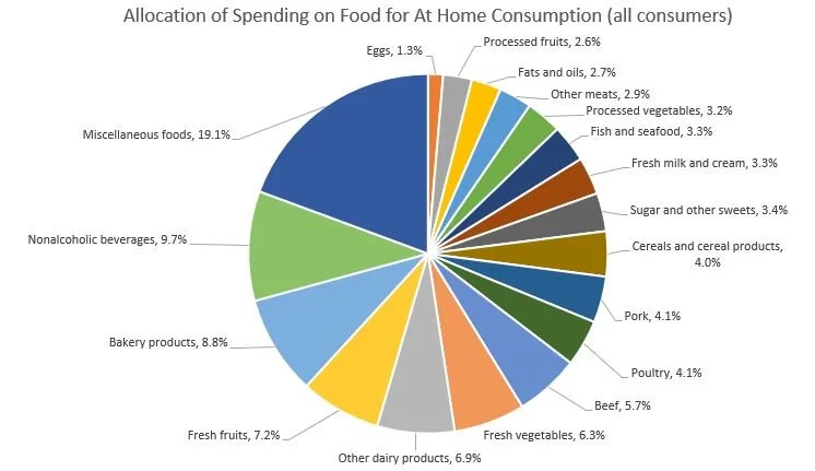
According to these data, on average about 43.6% of spending is on food to be consumed away from home (e.g., at restaurants), whereas 56.4% is spending for food to be consumed at home (e.g., spending at grocery stores). The BLS does not segregate data on spending on food away from home by the type of food, but it does so for spending on food to be consumed at home. Of the spending on food to be consumed at home (e.g., spending at grocery stores), the figure below shows the breakdown for the “average” food consumer. 19.1% of “at home” food spending is for “miscellaneous foods” and the next biggest category is nonalcoholic beverages (9.7%) and then bakery products (8.8%). Combined, all meat products including beef, pork, poultry, and fish account for 21.6% of at home food spending, and all dairy products account for another 10.2%.

The main reason for delving into these data is that they provide information on regional differences in food spending patterns. To explore these issues, I calculated the at food expenditure shares for each of the nine census regions, and then calculate the percent difference in expenditure share for a given region compared to the “average” consumer in the U.S. Here are some breakdowns, starting first with spending on beef as a share of all spending on food at home.

Differences in Spending on Beef by Region.

Consumers in the South West Central region (Arkansas, Louisiana, Oklahoma, and Texas) allocate 16.2% more of their at-home food budget to beef than does the national average food consumer, whereas on the other extreme, New England consumers (in Connecticut, Maine, Massachusetts, New Hampshire, Rhode Island, Vermont) allocate about 8.7% less of their food budget to beef than does the national average food consumer.

The following shows similar figures for pork and poultry. Whereas consumers in the Upper Midwest allocates a higher than average share of their food at home food budget to beef and pork, consumers there allocate 21.1% less of their food at home budget to poultry as compared to the average national food consumer.

Differences in Spending on Pork by Region

Differences in Spending on Poultry by Region.

Turning from meat items, here is data on relative spending on fresh fruits and fresh vegetables by region, which is higher in the West and New England.

Differences in Spending on Fresh Fruit by Region.

Differences in Spending on Fresh Vegetables by Region.

What about items that are often considered “unhealthy” like sugar and sweets and fats and oils? Spending on sugar and sweets is 27.3% higher in the Mountain region as compared to the average consumer, and spending on oils and fats is relatively highest in the East South Central Region.

Differences in Spending on Sugar and Sweets by Region.

Differences in Spending on Fats and Oils by Region.

The BLS CES reports spending on alcoholic beverages as a separate category from food at home or food away from home. Across all consumers, about 7% of food spending (either at home or away) is on alcoholic beverages. The variation across region is shown below. Spending on alcohol (as a share of total food spending) is positively correlated with spending on fresh fruits and fresh vegetables (as a share of spending on food at home), as alcohol spending is highest in the West and New England.

Differences in Spending on Alcohol by Region.

Finally, here is spending on food away from home as a share of total food spending. Consumers in the South West Central Region (Arkansas, Louisiana, Oklahoma, and Texas) and in the West spend 4% more on food away from home as a share of total food spending as compared to the average food consumer.

Differences in Spending on Food Away from Home by Region.

Readers who want to further explore the differences in regional spending patterns can access the BLS CES data here.

*The USDA Economic Research Service (ERS) reports data on per-capita “consumption” (this is actually “disapperance data, which infers consumption based on production, minus exports, plus imports, plus or minus net change in storage), but this is only at the national level. There are some other datasets which provide more local information on food purchases or consumption, but they are proprietary. Examples include grocery store scanner data by Nielsen or IRI. There are publicly available data, like the National Health and Nutrition Examination Survey (NHANES), which have information on location and food consumption, but it often requires significant data analytic abilities or special permission to make use of these data to explore state or regional trends.

Food Environment or Preferences?

Do poorer people eat unhealthily because they don’t have access to grocery stores and fresh fruits and vegetables (and are more easily able grab fast food or convenience store options), or is it because their preferences for healthy food differs from higher income households? In a sense, this is a question of nature vs. nurture applied to healthiness of food consumption, and it is a lively debate related to questions about food deserts, convenience store regulations, zoning, and more.

This interesting and rigorous paper (gated version here) on the topic by Hunt Allcott, Rebecca Diamond, Jean-Pierre Dube, Jessie Handbury, Ilya Rahkovsky, and Molly Schnell was recently published on the topic in the Quarterly Journal of Economics. I blogged about this paper a couple years ago, but I mentioned again now that it’s been revised and put through the rigors of the peer-reviewed process, and because the implications are quite important. Here’s the abstract:

“We study the causes of “nutritional inequality”: why the wealthy eat more healthfully than the poor in the United States. Exploiting supermarket entry and household moves to healthier neighborhoods, we reject that neighborhood environments contribute meaningfully to nutritional inequality. We then estimate a structural model of grocery demand, using a new instrument exploiting the combination of grocery retail chains’ differing presence across geographic markets with their differing comparative advantages across product groups. Counterfactual simulations show that exposing low-income households to the same products and prices available to high income households reduces nutritional inequality by only about ten percent, while the remaining 90 percent is driven by differences in demand. These findings counter the argument that policies to increase the supply of healthy groceries could play an important role in reducing nutritional inequality.”

These findings suggest efforts to eliminate food desserts or to constrain offerings of convenience stores are likely to have minimal effects. This paper shows, like some of my work, that higher- income households tend to eat healthier than lower-income households. Want lower income people to eat healthier? Then, we probably need to think about ways to increase their incomes. Another possible solution, albeit difficult to successfully and cost-effectively implement, is nutrition and health education.

Time to give thanks for affordable and sustainable turkey

That’s the title of an article I just wrote for The Conversation.

Here’s the whole thing:

Americans will eat about 210 million turkeys this year, amounting to over 16 pounds per person. Much of that will be eaten on Thanksgiving Day.

Over time, our Thanksgiving meal has become considerably more affordable. Turkey will probably average about US$1.40 per pound across the country in November 2019, which is less than half the price consumers were paying for turkey in the 1970s in inflation-adjusted terms.

How has turkey become so much more affordable? It turns out there isn’t a single factor, but rather a web of innovations.

The truth about turkey

It’s worth dispelling a few myths about the turkey industry first.

All farm-raised turkeys are supposed to be hormone-free.

For one thing, turkeys aren’t given any added growth hormones – doing so is illegal. It’s also illegal to sell turkey with antibiotic residues.

Also, all turkeys are raised cage-free in large, open barns.

Why aren’t more turkeys raised free-range, which means they are allowed to move outside with some freedom? It might initially sound great for turkeys to live outdoors – unless it’s snowing or raining or above 100 degrees.

It might also be fine unless there are roaming hawks, coyotes, dogs – or even wild birds. In 2015, the turkey industry was devastated by avian influenza that cost producers $225 million. Many experts believe the outbreak was caused by the introduction and spread of the disease by wild birds.

Bringing turkeys indoors allows farmers to protect the animals from weather, predators and disease, and it also enables farmers to more closely monitor their diets and health.

Spending less, eating more

Due to innovations in housing and genetics, it now takes less time and less feed to grow a turkey to market weight than it used to.

In the 1970s, the U.S. raised an average of about 125 million turkeys per year and produced about 1.9 billion pounds of turkey meat each year, meaning each turkey produced a little over 15 pounds of meat. This year, the country is projected to produce almost 25 pounds per bird.

This has led to increased affordability for Thanksgiving meals, but it has also had important implications for sustainability.

Let’s suppose Americans want to enjoy the amount of turkey we will actually consume as a nation this year – about 5.3 billion pounds – but we wanted to do that using 1970s technology. How many more turkeys would we need today had we not innovated to increase the amount of meat per bird from 15 to 25 pounds?

The answer is 132 million more turkeys.

That’s 132 million more turkeys that would have emitted waste, created greenhouse gas emissions and required water and feed. Growing that extra feed would have required more land, fertilizer and pesticides.

We were able to save those extra 132 million turkeys because we were innovative and used scientific developments and trial and error to figure out how to satisfy the wants of a much larger population using fewer of our natural resources.

That’s something to be thankful for.

Potential Economic Impacts of African Swine Fever (ASF)

African Swine Fever (ASF) is a viral disease that affects domestic and wild pigs. ASF is highly infectious and is fatal for pigs. Unfortunately, ASF has been ravaging the Chinese pork industry, which is by far the largest in the world. Some estimates suggest more pigs in China have died from ASF than exist in all of the United States. ASF does not cause illness in humans, but border security has been ramped up in the U.S. to make sure the virus doesn’t enter and hit our producers.

The other day I was asked about the potential economic impacts if ASF hit the United States. To answer the question, I constructed a fairly simply model of the U.S. pork industry (see details here). The basic idea is this that if ASF hit the U.S., the quantity of pork supplied would fall. This would, of course, result in less pork on the market and would result in an increase in price of hogs and pork for consumers. I considered three possible scenarios: a 10%, 25%, and 50% reduction in the quantity of U.S. pork supplied as potential outcomes of ASF. Of course, there are other possible impacts. It is likely that foreign buyers of U.S. pork might shut off imports from the U.S. to protect their own domestic herds. Thus, I also considered what happens if all foreign buyers of U.S. pork stopped importing. Finally, even though the disease does not affect humans, domestic consumers may choose to cut back if ASF hit the domestic herd; I thus considered a 10% reduction in consumer willingness-to-pay for pork.

Here are the possible impacts I calculate.

First, consider the impacts if only U.S. domestic supply is affected but foreign and U.S. consumers do not change their preferences. In the mildest scenario (a 10% supply reduction), both U.S. consumers and U.S. hog producers would lose about $1 billion/year. In the worst-case scenario considered (a 50% supply reduction), both U.S. producers and consumers would be worse off by almost $5 billion/year.

Now, what happens if foreign buyers of U.S. pork decide to stop buying? Over 20% of U.S. domestic production is exported, so the effects aren’t trivial. The estimates under the three supply reduction scenarios and a 100% reduction in foreign quantity demanded are shown below. Now, the worst-case scenario (a 50% supply reduction) results in an almost $7 billion/year loss for U.S. producers. The impacts on U.S. consumers are somewhat muted because there is now more supply on the U.S. market for U.S. consumers since foreign buyers are no longer buying, and as a result their losses aren’t as severe as in the above table.

Finally, consider the worst of all impacts. Supply in the U.S. falls (by either 10%, 25% or 50%), foreign buyers reduce their quantity demanded by 100%, and U.S. consumers also reduce their willingness-to-pay by 10%. Now, both U.S. producer and consumer impacts vary from about $4 to about $8 billion/year.

Don’t like my estimates or assumptions? Feel free to modify my model or mess around with the spreadsheet I used to create these results.

Spending on Beef over Time

Meat demand has been a frequent topic on this blog (e.g., see here, here, here, or here). As some of the previous posts indicate, “demand” is a hard thing to measure. A slightly easier thing to measure is spending. As it turns out, the Bureau of Labor Statistics (BLS) has been tracking consumer spending at the household level on food at home in a number of categories, including beef, pork, and poultry, in their annual Consumer Expenditure Survey.

Using these data, I constructed the following animation showing the relationship between spending on beef and total household expenditures by quintiles of income.

The figure shows, at any point in time, higher income households (or those with greater total spending) spend more on beef than lower income households (or those with less total spending). In econ-speak, beef is a “normal” good. However, for any given income (or total spending) level, spending on beef has fallen precipitously since 1984 (all figures are in inflation-adjusted 2017 dollars). The change over time is most dramatic for the higher income/spending households. In 1984, the lowest and highest quintile income households spent $265 and $681 per year (in 2017 dollars), respectively, on beef for consumption at home. By 2017, these figures had fallen to $158 and 352, respectively.

These data could be reflective of downward demand shift - i.e., consumers willing to pay less for each pound of beef than they were in the past. Other possible explanations for the downward decline in spending include changing beef prices over this period, changing household demographics (the average number of people in today’s households is slightly smaller today than in the mid 1980s; fewer people normally means less spending), other protein sources, such as poultry, becoming relatively less expensive or more attractive, a shift toward more food spending away from home (the BLS only tracks spending for individual food categories for food eaten at home), and more.

How do the data in the above figure square with measures of demand (such as these constructed by Glynn Tonsor), which show no clear trend in beef demand since the early 1990s? Well, as I mentioned above, spending isn’t “demand” because while the figure controls for income, it doesn’t control for prices. Another possible explanation is that the data in the figure above are for households, while aggregate demand statistics like those created by Tonsor are calculated nationally. It is possible for total aggregate demand to rise even if each individual household’s demand is falling if population is increasing and more households are being added. That is, in fact, what has happened. There were about 86 million households in the US in 1984. Today there are about 128 million households.