Worrying Trends with Farm Surveys

“Response rates on [USDA-National Agricultural Statistics Survey] crop acreage and production surveys have been falling in recent decades (Ridolfo, Boone, and Dickey, 2013). From response rates of 80-85 percent in the early 1990s, rates have fallen below 60 percent in some cases (Figure 1). Of even greater concern, there appears to an acceleration in the decline in the last 5 years or so, suggesting the possibility that this decline reflects a long-term permanent change.”

That's from an interesting (yet worrying) article by the USDA chief economist Robert Johansson along with Anne Effland, and Keith Coble at farmdocdaily. 

Why does this matter?

Responses to these surveys form the basis of what we think we know about, for example, how much farmland is in production, how much corn vs. soybeans is planted in a given year, the extent to which wheat yields are trending upward, and more.  It's hard to understate how much of what we think we know about the state of U.S. agriculture stems from these surveys.   For examples, I used these data in my article in the New York Times to describe the gains in farm productivity over time;  economists use the data to try to predict the possible effects of climate change on crop yields and farm profitability; the data are used to try to figure out how farmer's planting decisions respond changes in crop prices (which provide estimates of the elasticity of supply, which feed into various models that inform policy makers), and much more.

The concern with falling response rates is that the farmers who respond may be different than the one's who don't in a way that biases our understanding of crop acreage and production.  The authors write:  

“Reduced response rates can potentially introduce bias or error to the estimates released by USDA. For example bias may occur if higher yielding farms drop out. Reduced response will almost assuredly introduce error to the estimates making them noisier and randomly more inaccurate. This will be most noticeable in county estimates. ”

The authors go on to note that some farm program payments depend on county-level yield estimates (which the above note notes are now less reliable).  As such, this isn't just some academic curiosity, but an issue that could literally affect millions of taxpayer dollars.    

The problem of declining response rates isn't just with farmers.  This paper, appropriately titled "Household Surveys in Crisis", points out it is an issue with other government surveys of households as well. These are the surveys that attempt to provide statistics on people's incomes, employment, and so forth.

The solutions to these problems are not obvious or easy.  Here is the authors' take:

“Some research suggests that tailoring survey approaches to differing audiences within the survey population could improve response rates (Anseel et al., 2010). Other data sources like remote sensing, weather data, modeling, machine data, or integrated datasets may also be useful in providing additional information. NASS already makes use of some of these other data sources and methods in developing estimates, but as a supplement, not a replacement, for survey data. Further use of such sources is costly. For now, the best approach remains encouraging greater producer response.”

How risk averse are you?

Economists have long been interested in trying to figure out people's tolerance for risk.  Such information is useful in predicting, for examples, which crops farmers will plant, which stocks investors will buy, how much insurance is bought, how much of a premium one is willing to pay for organic food, and how fast people drive.  Of course, we don't expect all people to have the same risk preferences, so for decades economists have sought to identify tools and methods that will allow them to discover different people's levels of risk aversion.

One of the most popular techniques is the so-called Holt and Laury (H&L) multiple price list (MPL) based on this paper in the American Economic Review.  As of this writing, the paper has been cited 3,900 times according to googlescholar, making it one of the most cited economic papers published in the last 15 years.  The approach requires people to make a choice between a relatively safe lottery (e.g., 10% chance of $2 and a 90% chance of $1.60) and a relatively risky lottery (e.g., 10% chance of $3.85 and a 90% chance of $0.10).  Then, the subject repeats the choice except the probability of the higher payoffs increases.  This process is repeated again and again about 10 times until one gets to the very easy choice between 100% chance of $2 and 100% chance of $3.85 (If you don't know which of those you prefer, give me a call.  We need to talk).  One very crude measure of risk aversion is simply the number of times a person chooses the relatively safe lottery over the relatively risky lottery.  

The H&L method is relatively easy to use, which goes a long way toward explaining it's popularity.

With all that as a backdrop, I'll point you to a new paper I published with Andreas Drichoutis in the Journal of Risk and Uncertainty. We point out an important problem with using the H&L method as a measure of risk aversion and propose a new, yet equally easy to use, MPL that helps solve the problem.  If you're not an academic economist, the rest of this may get a bit wonky, but here goes:

“In what follows, we show that H&L’s original MPL is, perhaps ironically, not particularly well suited to measuring the traditional notion of risk preferences — the curvature of the utility function. Rather, it is likely to provide a better approximation of the curvature of the probability weighting function. We then introduce an alternative MPL that has exactly the opposite property. By combining the information gained from both types of MPLs, we show that greater prediction performance can be attained.”

Here is one of the main critiques of H&L, which relates to whether people weight probabilities non-linearly (the parameter γ is a measure of the extent to which probabilities are "distorted").

“Now, consider a simple example where individuals have a linear utility function (i.e., they are risk neutral in the traditional sense), U(x) = x. With the traditional H&L task, a risk neutral person with U(x) = x and γ = 1 would switch from option A to B at the fifth decision task. However, if the person weights probabilities non-linearly, say with a value of γ = 0.6, then they would instead switch from option A to B at the sixth decision task. Thus, in the original H&L decision task, an individual with γ = 0.6 will appear to have a concave utility function (if one ignores probability weighting) even though they have a linear utility function, U(x) = x. The problem is further exasperated as γ diverges from one. Of course in reality, people may weight probabilities non-linearly and exhibit diminishing marginal utility of earnings, but the point remains: simply observing the A-B switching point in the H&L decision task is insufficient to identify the shape of U(x) and the shape of w(p). The two are confounded. While it is possible to use data from the H&L technique to estimate these two constructs, U(x) and w(p), ex post, we argue that more information is contained about w(p) than U(x) in the original H&L MPL.”

The other problem we point out with the H&L approach is that it provides very little information about the shape of U(x) as only four dollar amounts are used in the design (and only two differences are uniquely identified).  Instead, 10 different probabilities are used, which provides much more information about the shape of γ.  What can one do about this if they truly want to know about the shape of U(x)?  We suggest a new kind of payoff-varying MPL.

“Given the preceding discussion, one might ask if there is a simple way to use a MPL that yields more information about U(x) and, at least in some special cases, avoids the confound between w(p) and U(x)? One can indeed achieve such an outcome by following an approach like the one used by Wakker and Deneffe (1996) in which probabilities are held constant. Using this insight, we modify the H&L task such that probabilities remain constant across the ten decision tasks and instead change the monetary payoffs down the ten tasks. ”

I'm under no allusion that our new MPL will become nearly as popular as the original H&L task.  But, if we even get one-tenth their number of citations, I'll be thrilled.

What's going on in your brain?

Ever wonder why you choose one food over another?  Sure, you might have the reasons you tell yourself for why you picked, say, cage vs. cage free eggs. But, are these the real reasons?

I've been interested in these sorts of questions for a while, and along with several colleagues, have turned to a new tool - functional magnetic resonance imaging (fMRI) - to peak people inside people's brains as they're choosing between different foods.  You might be able to fool yourself (or survey administrators) about why you do something, but you're brain activity doesn't lie (at lest we don't think it does).  

In a new study that was just released by the Journal of Economic Behavior and Organization,  my co-authors and I sought to explore some issues related to food choice.  The main questions we wanted to know were: 1) does one of the core theories for how consumers choose between goods of different qualities (think cage vs cage free eggs) have any support in neural activity?, and 2) after only seeing how your brain responses to seeing images of eggs with different labels, can we actually predict which eggs you will ultimately choose in a subsequent choice task?   

Our study suggests the answers to these two questions are "maybe" and "yes".  

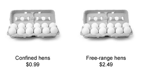
First, we asked people to just look at eggs with different labels while they were laying in the scanner.  The labels were either a high price, a low price, a "closed" production method (caged or confined), or an "open" production method (cage free or free range), as the below image suggests.  As participants were looking at different labels we observed whether blood flow increased or decreased to different parts of the brain when seeing, say, higher prices vs. lower prices.  

We focused on a specific areas of the brain, the ventromedial prefrontal cortex (vmPFC), which previous research had identified as a brain region associated with forming value.  

What did his stage of the research study find?  Not much.  There were no significant differences in brain activation in the vmPFC when looking at high vs. low prices or when looking at open vs. closed production methods.  However, there was a lot of variability across people.  And, we conjectured that this variability across people might predict which eggs people might choose in a subsequent task.  

So, in the second stage of the study, we gave people a non-hypothetical choice like the following, which pitted a more expensive carton of eggs produced in a cage free system against a lower priced carton of eggs from a cage system.  People answered 28 such questions where we varied the prices, the words (e.g., free range instead of cage free), and the order of the options.  One of the choices was randomly selected as binding and people had to buy the option they chose in the binding task.  

Our main question was this: can the brain activation we observed in the first step, where people were just looking at eggs with different labels predict which eggs they would choose in the second step?

The answer is "yes".  In particular, if we look at the difference in the brain activation in the vmPFC when looking at eggs with a "open" label vs. an "closed" label, this is significantly related to the propensity to choose the higher-priced open eggs over the lower-priced closed eggs (it should be noted that we did not any predictive power from the difference in vmPFC when looking at high vs. low priced egg labels).  

Based on a statistical model, we can even translate these differences in brain activation into willingness-to-pay (WTP) premiums:

Here's what we say in the text:

“Moving from the mean value of approximately zero for vmPFCmethodi to twice the standard deviation (0.2) in the sample while holding the price effect at its mean value (also approximately zero), increases the willingness-to-pay premium for cage-free eggs from $2.02 to $3.67. Likewise, moving two standard deviations in the other direction (-0.2) results in a discount of about 38 cents per carton. The variation in activations across our participants fluctuates more than 80 percent, a sizable effect that could be missed by simply looking at vmPFCmethod value alone and misinterpreting its zero mean as the lack of an effect. ”

Does Diet Coke Cause Fat Babies?

O.k., I just couldn't let this one slide.  I've seen the results of this study in JAMA Pediatrics discussed in a variety of news outlets with the claim that researchers have found a link between mothers drinking artificially sweetened beverages and the subsequent weight of their infants.

I'm going to be harsh here, but this sort of study represents everything wrong with a big chunk of the nutritional and epidemiology studies that are published and how they're covered by the media.  

First, what did the authors do?  They looked at the weight of babies one year after birth and looked at how those baby weights correlated with whether (and how much) Coke and Diet Coke the mom drank, as indicated in a survey, during pregnancy.  

The headline result is that moms who drank artificially sweetened beverages every day in pregnancy had slightly larger babies, on average, a year later than the babies from moms who didn't drink any artificially sweetened beverages at all.  Before I get to the fundamental problem with this result, it is useful to look at a few more results contained in the same study which might give us pause.

• Mom's drinking sugar sweetened beverages (in any amount) had no effect on infants' later body weights.  So drinking a lot of sugar didn't affect babys' outcomes at all but drinking artificial sweeteners did?
• The researchers only found an effect for moms who drank artificially sweetened beverages every day.  Compared to moms who never drink them, those who drink diet sodas less than once a week actually had lighter babies! (though the result isn't statistically significant).  Also, moms drinking artificially sweetened beverages 2-6 times per week had roughly the same weight babies as moms who never drank artificially sweetened beverages.  In short, there is no evidence of a dose-response relationship that one would expect to find if there was a causal relationship at play.  

And, that's the big issue here: causality.  The researchers have found a single statistically significant correlation in one of six comparisons they made (three levels of drinking compared to none for sugar sweetened beverages and for artificially sweetened beverages).  But, as the researchers themselves admit, this is NOT a casual link (somehow that didn't prevent the NYT editors from using the word "link" in the title of their story).  

Causality is what we want to know.  An expecting mother wants to know: if I stop drinking Diet Coke every day will that lower the weight of my baby?  That's a very different question than what the researchers actually answered: are the types of moms who drink Diet Coke every day different from moms who never drink Diet Coke in a whole host of ways, including how much their infants weigh?  

Why might this finding be only a correlation and not causation? There are a bunch of possible reasons.  For example, moms who expect their future children might have weight problems may choose to drink diet instead of regular.  If so, the the moms drinking diet have selected themselves into a group that is already likely to have heavy children.  Another possible explanation: moms who never drink Diet Cokes may be more health conscious overall.  This is an attitude that is likely to carry over to how they feed and raise their children which will affect their weight in ways that has nothing to do with artificially sweetened beverages.

Fortunately economics (at least applied microeconomics) has undergone a bit of credibility revolution.  If you attend a research seminar in virtually any economist department these days, you're almost certain to hear questions like, "what is your identification strategy?" or "how did you deal with endogeneity or selection?"  In short, the question is: how do we know the effects you're reporting are causal effects and not just correlations.  

Its high time for a credibility revolution in nutrition and epidemiology.  

Economics of Food Waste

There seems to be a lot of angst these days about food waste.  Last month, National Geographic focused a whole issue on the topic.  While there has been a fair amount of academic research on the topic, there has been comparatively little on the economics of food waste.  Brenna Ellison from the University of Illinois and I just finished up a new paper to help fill that void.

Here's the core motivation.

“Despite growing concern about food waste, there is no consensus on the causes of the phenomenon or solutions to reduce waste. In fact, many analyses of food waste seem to conceptualize food waste as a mistake or inefficiency, and in some popular writing a sinful behavior, rather than an economic phenomenon that arises from preferences, incentives, and constraints. In reality consumers and producers have time and other resource constraints which implies that it simply will not be worth it to rescue ever last morsel of food in every instance, nor should it be expected that consumers with different opportunity costs of time or risk preferences will arrive at the same decisions on whether to discard food”

So, what do we do?

First, we create a conceptual model based on Becker's model of household production to show that waste is indeed "rational" and responds to various economic incentives like time constraints, wages, and prices.  

We use some of these insights to design a couple empirical studies.  One problem is that it is really tough to measure waste.  And, people aren't likely to be very accurate at telling you, on a survey, how much food they waste.  Thus, we got a bit creative and came up with a couple vignette designs that focused on very specific situations.  

In the first study, respondents were shown the following verbiage.  The variables that were experimentally varied across people are in brackets (each person only saw one version).  

“Imagine this evening you go to the refrigerator to pour a glass of milk. While taking out the carton of milk, which is [one quarter; three quarters] full, you notice that it is one day past the expiration date. You open the carton and the milk smells [fine; slightly sour]. [There is another unopened carton of milk in your refrigerator that has not expired; no statement about replacement]. Assuming the price of a half-gallon carton of milk at stores in your area is [$2.50; $5.00], what would you do?”

More than 1,000 people responded to versions of this question with either "pour the expired milk down the drain" or "go ahead and drink the expired milk."  

Overall, depending on the vignette seen, the percentage of people throwing milk down the drain ranged from 41% to 86%.

Here are how the decision to waste varied with changes in the vignette variables.

The only change that had much impact on food waste was food safety concern.  The percentage of people who said they'd discard the milk fell by 38.5 percentage points, on average, when the milk smelled fine vs. sour.  The paper also reports how these results vary across people with different demographics like age income, etc.

We conducted a separate study (with another 1,000 people) where we changed the context from milk to a meal left-over.  Each person was randomly assigned to a group (or vignette), where they saw the following (experimentally manipulated variables are in brackets).

“Imagine you just finished eating dinner [at home; out at a restaurant]. The meal cost about [$8; $25] per person. You’re full, but there is still food left on the table – enough for [a whole; half a] lunch tomorrow. Assuming you [don’t; already] have meals planned for lunch and dinner tomorrow, what would you do?”

People had two response options: “Throw away the remaining dinner” or “Save the leftovers to eat tomorrow”.

Across all the vignettes, the percent throwing away the remaining dinner ranged from 7.1% to 19.5%.  

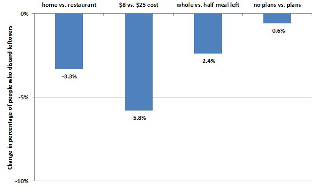
Here are how the results varied with changes in the experimental variables.

Meal cost had the biggest effect.  Eating a meal that cost $25/person instead of one that cost only $8/person reduced the percentage of people discarding the meal by an average of 5.8 percentage points.  People were also less likely to throw away home cooked meals than restaurant meals.  

There's a lot more in the paper if you're interested.