Do you plan to spend more or less eating out in the next two weeks?

The title of this post is based on a question I ask of food consumers every month in my Food Demand Survey (FooDS).  If I had to guess your response, I'd go with "spend less."  Why?  Because every month, for almost four years, that has been the average response to the question (the exact question is: "Do you expect to spend more or less on food bought during grocery shopping in the next two weeks as compared to the previous two weeks?" and response categories are: "I plan to spend about . . . 10% less, 5% less, the same, 5% more, or 10% more").   

Here is the problem with the above results.  They are almost certainly false.  If people are continually, month after month, saying they plan to spend less on food away from home, the cumulative effect would ultimately be a negative amount of spending.  

Moreover, another question I ask on the survey relates to how much the respondent says they spend (in dollars) on food away from home (exact question wording: "What has been you (or your household's) usual WEEKLY expense for meals or snacks from restaurants, fast food places, cafeterias, carryout or other such places?"  The response categories are: less than $20, $20-$39, . . . $140-$159, $160 or more).  

In the most recent issue of FooDS, we estimate the average level of spending on food away from home in January 2017 was $53.26/week.  The average answer from the previous month (December 2016) was $50.89/week.  So, in terms of stated expenditure, there was a $53.26-$50.89=$2.37 increase (or a (2.37/50.89)*100=4.66% increase). Yet, (and here is the problem), In December 2016, people said they planned to reduce spending on food away from home by, on average, -0.59%, and in January 2017, they said they plan to reduce spending on food away from home by, on average, -1.47%.

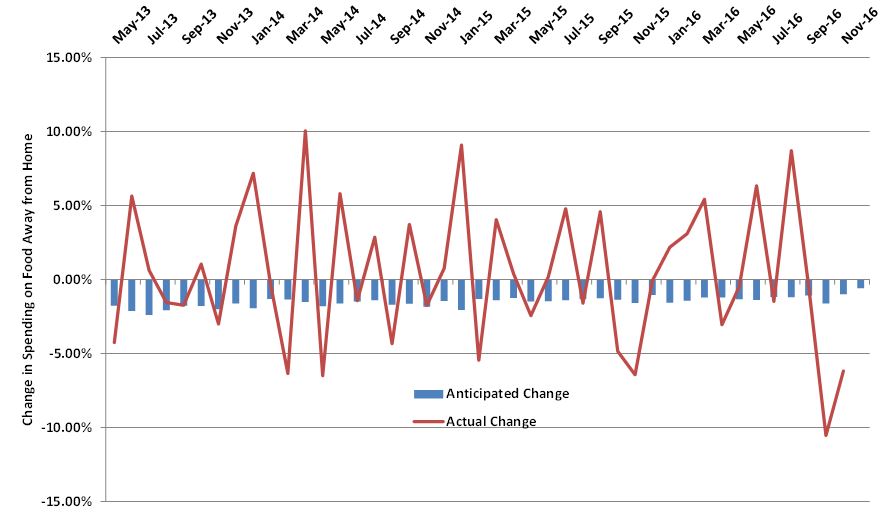
Here is what I get if I calculate "actual" changes in reported levels of spending on food away from home against people's stated plans to increase or decrease spending (the blue bars are the same blue bars as in the above graph, they just look different because the vertical axis has been re-scaled).       

So, what is going on here?  One possible answer is that consumers suffer from a type of self-control problem.  We tell ourselves we want to reduce the amount we're spending on food away from home in the future.  But, when the future arrives, we forget our plans and have fun eating out with our friends and keep spending as usual.  If this is correct, eating out is a sort of "guilty pleasure" - something we enjoy but wish we could force our future selves to cut back on.     

The propensity of an individual to say they plan to reduce spending on food away from home relates to a variety of demographic variables (even after controlling for the month-to-month effects that may be driving changing spending patterns).  Income is a major determinant.  Lower income people are much more likely to say they plan to reduce spending on food away from home than higher income respondents.  Indeed, for the highest income households, there is no consistent upward or downward bias in planned spending patterns for food away from home.  Other (smaller) determinants include gender, age, and participation in food assistance programs with women, older, and SNAP participants being more likely to say they plan to reduce spending on food away from home.

A less nefarious explanation for the above phenomenon might be that our survey is conducted in the middle of the month, and if people are paid at the beginning of the month (or at the end of the previous month), then there might be less remaining in the food budget for "splurges" like spending on food away from home by the time the middle of the month arises and they rationally plan to spend less in the following two weeks.  

I doubt this is true for two reasons.  The first is that results from other surveys back up the "self control" explanation.  For example, this article in the Wall Street Journal a couple years ago pointed to a survey of higher income consumers that asked what kept them from saving more money each month.  The most common answer, given by 68% of respondents, was "dining out".  The second reasons is that we observe no such phenomenon in our survey for stated changes in spending on food AT home.  Here is the average response each month for how consumers expect to change spending on food at home.  As can be seen, the value goes up and down and is neither consistently negative or positive.     

If you have other explanations for why people consistently say they plan to spend less eating out next month, I'd love to hear them.

Economics and Obesity Policy

The International Journal of Obesity just released a a short review paper I was invited to write, which discusses the economics of policies aimed at reducing obesity. In the paper, I touch on the economic approach for thinking about government intervention in this space and whether there are market failures that would justify intervention.  I then move on to discuss a variety of specific issues that are often discussed in relation to obesity such as farm policy, soda taxes, healthy food subsidies, food assistance programs (and proposed restrictions on them), and information policies. 

Here is the conclusion:

“This article presented a somewhat pessimistic view on the ability of government policy to substantively influence obesity prevalence. Obesity is a complicated and multifaceted issue. So too are the effects of anti-obesity policies. One response is to argue for an all-out ‘war’ on obesity. It probably is true that government policy mandating what farms grow, restricting the
supply and type of food to consumers, and controlling prices, offerings and advertisements by food manufacturers could reduce obesity prevalence. But, is this the type of coercive
society in which we would like to live? Society faces very real tradeoffs between economic freedom, technological progress, and obesity prevalence. These sorts of tradeoffs are unfortunate, but they reflect very real constraints to effective economic policy making.”

My paper joins several others that critically evaluate anti-obesity policies.

Unanticipated Effects of Soda Tax, example 1037

On the surface the logic of a soda tax seems simple: raise the price of an unhealthy food, people consume less, and public health improves.  But, as I've pointed out again and again on this blog, the story is much less simple than it first appears.  

First, even if we believe people suffer from various behavioral biases, higher prices almost certainly make people worse off.  Second, when we raise the price of one unhealthy thing, people might substitute to consume other unhealthy things.  Third, if the tax is just added at the checkout counter and not on the shelf display, it may not have nearly the effect on purchase behavior as assumed.  Forth, if people know the reason for the tax, some may "protest" and buy more instead.  Fifth, the projected weight loss from such taxes often relies on unreasonable rules of thumb like 3500kcal=1lb. Six, even when taxes have an effect, the causal impact may arise more from an "information effect" rather than a "price effect."  Seventh, such taxes may induce unanticipated effects because of how sellers respond to the policy.  Finally, soda taxes are regressive - having a proportionally larger effect on on lower income households (see also my co-authored paper on effects of "unhealthy" food taxes more generally).

Now, comes this new paper in the American Journal of Agricultural Economics by Emily Wang, Christian Rojas, and Francesca Colantuoni, which incorporates the insight that some households are more likely to respond to promotions and to store.  The abstract:

“We apply a dynamic estimation procedure to investigate the effect of obesity on the demand for soda. The dynamic model accounts for consumers’ storing behavior, and allows us to study soda consumers’ price sensitivity (how responsive consumers are to the overall price) and sale sensitivity (the fraction of consumers that store soda during temporary price reductions). By matching store-level purchase data to county-level data on obesity incidence, we find higher sale sensitivity in populations with higher obesity rates. Conversely, we find that storers are less price sensitive than non-storers, and that their price sensitivity decreases with the obesity rate. Our results suggest that policies aimed at increasing soda prices might be less effective than previously thought, especially in areas where consumers can counteract that price increase by stockpiling during sale periods; according to our results, this dampening effect would be more pronounced precisely in those areas with higher obesity rates.”

Worrying Trends with Farm Surveys

“Response rates on [USDA-National Agricultural Statistics Survey] crop acreage and production surveys have been falling in recent decades (Ridolfo, Boone, and Dickey, 2013). From response rates of 80-85 percent in the early 1990s, rates have fallen below 60 percent in some cases (Figure 1). Of even greater concern, there appears to an acceleration in the decline in the last 5 years or so, suggesting the possibility that this decline reflects a long-term permanent change.”

That's from an interesting (yet worrying) article by the USDA chief economist Robert Johansson along with Anne Effland, and Keith Coble at farmdocdaily. 

Why does this matter?

Responses to these surveys form the basis of what we think we know about, for example, how much farmland is in production, how much corn vs. soybeans is planted in a given year, the extent to which wheat yields are trending upward, and more.  It's hard to understate how much of what we think we know about the state of U.S. agriculture stems from these surveys.   For examples, I used these data in my article in the New York Times to describe the gains in farm productivity over time;  economists use the data to try to predict the possible effects of climate change on crop yields and farm profitability; the data are used to try to figure out how farmer's planting decisions respond changes in crop prices (which provide estimates of the elasticity of supply, which feed into various models that inform policy makers), and much more.

The concern with falling response rates is that the farmers who respond may be different than the one's who don't in a way that biases our understanding of crop acreage and production.  The authors write:  

“Reduced response rates can potentially introduce bias or error to the estimates released by USDA. For example bias may occur if higher yielding farms drop out. Reduced response will almost assuredly introduce error to the estimates making them noisier and randomly more inaccurate. This will be most noticeable in county estimates. ”

The authors go on to note that some farm program payments depend on county-level yield estimates (which the above note notes are now less reliable).  As such, this isn't just some academic curiosity, but an issue that could literally affect millions of taxpayer dollars.    

The problem of declining response rates isn't just with farmers.  This paper, appropriately titled "Household Surveys in Crisis", points out it is an issue with other government surveys of households as well. These are the surveys that attempt to provide statistics on people's incomes, employment, and so forth.

The solutions to these problems are not obvious or easy.  Here is the authors' take:

“Some research suggests that tailoring survey approaches to differing audiences within the survey population could improve response rates (Anseel et al., 2010). Other data sources like remote sensing, weather data, modeling, machine data, or integrated datasets may also be useful in providing additional information. NASS already makes use of some of these other data sources and methods in developing estimates, but as a supplement, not a replacement, for survey data. Further use of such sources is costly. For now, the best approach remains encouraging greater producer response.”

How risk averse are you?

Economists have long been interested in trying to figure out people's tolerance for risk.  Such information is useful in predicting, for examples, which crops farmers will plant, which stocks investors will buy, how much insurance is bought, how much of a premium one is willing to pay for organic food, and how fast people drive.  Of course, we don't expect all people to have the same risk preferences, so for decades economists have sought to identify tools and methods that will allow them to discover different people's levels of risk aversion.

One of the most popular techniques is the so-called Holt and Laury (H&L) multiple price list (MPL) based on this paper in the American Economic Review.  As of this writing, the paper has been cited 3,900 times according to googlescholar, making it one of the most cited economic papers published in the last 15 years.  The approach requires people to make a choice between a relatively safe lottery (e.g., 10% chance of $2 and a 90% chance of $1.60) and a relatively risky lottery (e.g., 10% chance of $3.85 and a 90% chance of $0.10).  Then, the subject repeats the choice except the probability of the higher payoffs increases.  This process is repeated again and again about 10 times until one gets to the very easy choice between 100% chance of $2 and 100% chance of $3.85 (If you don't know which of those you prefer, give me a call.  We need to talk).  One very crude measure of risk aversion is simply the number of times a person chooses the relatively safe lottery over the relatively risky lottery.  

The H&L method is relatively easy to use, which goes a long way toward explaining it's popularity.

With all that as a backdrop, I'll point you to a new paper I published with Andreas Drichoutis in the Journal of Risk and Uncertainty. We point out an important problem with using the H&L method as a measure of risk aversion and propose a new, yet equally easy to use, MPL that helps solve the problem.  If you're not an academic economist, the rest of this may get a bit wonky, but here goes:

“In what follows, we show that H&L’s original MPL is, perhaps ironically, not particularly well suited to measuring the traditional notion of risk preferences — the curvature of the utility function. Rather, it is likely to provide a better approximation of the curvature of the probability weighting function. We then introduce an alternative MPL that has exactly the opposite property. By combining the information gained from both types of MPLs, we show that greater prediction performance can be attained.”

Here is one of the main critiques of H&L, which relates to whether people weight probabilities non-linearly (the parameter γ is a measure of the extent to which probabilities are "distorted").

“Now, consider a simple example where individuals have a linear utility function (i.e., they are risk neutral in the traditional sense), U(x) = x. With the traditional H&L task, a risk neutral person with U(x) = x and γ = 1 would switch from option A to B at the fifth decision task. However, if the person weights probabilities non-linearly, say with a value of γ = 0.6, then they would instead switch from option A to B at the sixth decision task. Thus, in the original H&L decision task, an individual with γ = 0.6 will appear to have a concave utility function (if one ignores probability weighting) even though they have a linear utility function, U(x) = x. The problem is further exasperated as γ diverges from one. Of course in reality, people may weight probabilities non-linearly and exhibit diminishing marginal utility of earnings, but the point remains: simply observing the A-B switching point in the H&L decision task is insufficient to identify the shape of U(x) and the shape of w(p). The two are confounded. While it is possible to use data from the H&L technique to estimate these two constructs, U(x) and w(p), ex post, we argue that more information is contained about w(p) than U(x) in the original H&L MPL.”

The other problem we point out with the H&L approach is that it provides very little information about the shape of U(x) as only four dollar amounts are used in the design (and only two differences are uniquely identified).  Instead, 10 different probabilities are used, which provides much more information about the shape of γ.  What can one do about this if they truly want to know about the shape of U(x)?  We suggest a new kind of payoff-varying MPL.

“Given the preceding discussion, one might ask if there is a simple way to use a MPL that yields more information about U(x) and, at least in some special cases, avoids the confound between w(p) and U(x)? One can indeed achieve such an outcome by following an approach like the one used by Wakker and Deneffe (1996) in which probabilities are held constant. Using this insight, we modify the H&L task such that probabilities remain constant across the ten decision tasks and instead change the monetary payoffs down the ten tasks. ”

I'm under no allusion that our new MPL will become nearly as popular as the original H&L task.  But, if we even get one-tenth their number of citations, I'll be thrilled.